

Kubernetes
SaaS Infrastructure: Shared Kubernetes, Clusters or VMs?
Compare shared Kubernetes, tenant namespaces, dedicated clusters, and VMs for SaaS infrastructure. Learn how isolation, costs, and operations shape your choice.
Read field noteField notes / Latest
Engineering notes from operating open infrastructure: the failures, design decisions, and upstream work that make open infrastructure better.
Browse all field notesCompare shared Kubernetes, tenant namespaces, dedicated clusters, and VMs for SaaS infrastructure. Learn how isolation, costs, and operations shape your choice.
Read field note
Learn why backups alone don't guarantee recovery and how RTO, RPO, infrastructure dependencies, and recovery testing improve disaster readiness.
Read field note
Compare private AI inference, managed endpoints, and public AI APIs. Learn when data control, latency, model flexibility, and cost justify a change.
Read field note
How to choose between a consumption-priced API and dedicated capacity with some sample costs.
Short answer: Measure cost per successful outcome, meaning total spend divided by the outcomes your business actually accepted, and use that as your primary unit-economics number rather than relying on cost per token or cost per GPU hour alone. From there, work the drivers behind it: calls a cache or a smaller model could have handled, models larger than the task requires, bloated inputs and outputs, a prefix cache that isn't hitting, and batching settings nobody has tuned against your latency targets. If you run your own capacity, the equivalent calculation is the fully-loaded hourly cost of a capacity unit divided by the throughput that unit achieves at your required service level, which can be well below a published peak-throughput figure. Choosing between a consumption-priced API and dedicated capacity comes down to arithmetic over achieved throughput, demand variability, availability headroom, hardware efficiency and operating costs.
When an inference invoice grows faster than anyone forecast, the usual response is to go looking for a better rate, a cheaper provider or a smaller model. That isn't wasted effort, since procurement can shave a real percentage off a large bill, but it leaves alone the two variables that generally matter more: how many model calls your workflow makes to produce one useful result, and how much of each call was necessary in the first place.
Most of what determines the bill was settled long before it arrived, in design choices that remain open to revision. Revisiting them requires a cost model detailed enough to act on, meaning one that attributes spend to particular workflow steps and serving decisions rather than reporting a monthly total.
Most cost conversations muddle two different numbers, so it helps to pull them apart before anything else.
Cost per successful outcome is the operational metric, and it corresponds to what the business is actually buying: a ticket resolved, a document processed, a suggestion the developer accepted. It works as a primary unit-economics figure provided you read it alongside total spend and service-level performance, because a falling cost per outcome tells you little on its own if total spend is climbing, or if the improvement came from quietly missing latency targets.
The cost drivers are what produce that number: token volumes, retrieval and tool calls, cache behaviour, retry rates, and if you run your own capacity, hardware, energy, software, operations and achieved throughput.
On its own the metric tells you something has gone wrong without telling you where, while the drivers on their own will happily lead you into optimizing something that was never material. You need both, along with the relationship between them:
Cost per successful outcome = total cost of all attempts over a period ÷ number of successful outcomes over that period
The denominator does as much work here as the numerator, because retries, abandoned requests, responses nobody read and evaluation traffic all land in the numerator without contributing anything to the denominator. That's what separates the cost of an attempt from the cost of a business outcome.
Take a support triage workflow that retrieves relevant history, calls a model, invokes a tool and drafts a reply for an agent to accept or reject.
Step 1. Count tokens per attempt.
Embedding tokens bill at a different rate from generation tokens, so they get their own line rather than disappearing into the generation subtotal.
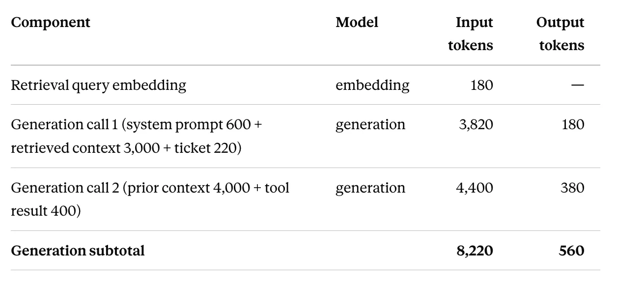
Step 2. Apply rates, including cached input.
The rates below are placeholders, so substitute your provider's. Assume $1.00 per million generation input tokens, $4.00 per million output tokens, $0.10 per million for cached input and $0.02 per million for embeddings, with 1,000 tokens of the generation input forming a stable prefix eligible for caching.
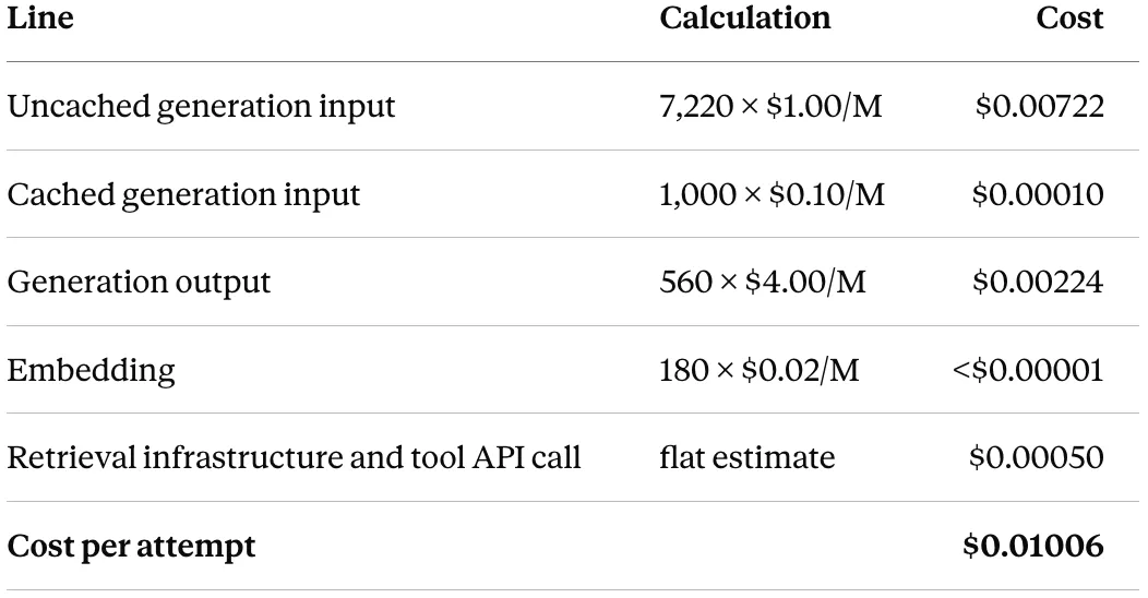
The embedding line is trivial at this volume but becomes material in retrieval-heavy workloads and any time you re-index, which is the argument for keeping it visible rather than folding it into a generation subtotal where nobody would notice it move.
Step 3. Apply retries and success rate.
The retry assumption needs stating precisely, because two reasonable readings produce different answers.
Assume 8% of initial runs need exactly one retry, and retries don't fail again. That gives 1.08 attempts per completed run. Assume 88% of completed runs produce a reply the agent accepts.
Cost per successful outcome = $0.01006 × 1.08 ÷ 0.88 = $0.0123
If failures can recur instead, with each attempt independently failing at probability p, the number of attempts follows a geometric distribution whose expected value is 1/(1−p) = 1/0.92 = 1.087, giving $0.0124. At an 8% failure rate that difference is small, though it widens quickly as the rate climbs, so it's better to establish which regime you're in before anyone builds a forecast on the number.
Taking the first assumption, an attempt costs $0.0101 while a successful outcome costs $0.0123, roughly 23% more, which at 20,000 outcomes a day works out to about $247 daily or $7,400 a month.
The space between those two figures is the part of the bill that token-level accounting hides, and it tends to respond to workflow changes rather than price negotiations.
The dedicated calculation has the same shape but a different numerator: the cost is a fully-loaded hourly rate for a capacity unit, and the denominator is what that unit actually delivers at your service level.
Step 1. Fully-loaded cost per capacity unit.
The figures below are illustrative, for one node of eight accelerators.
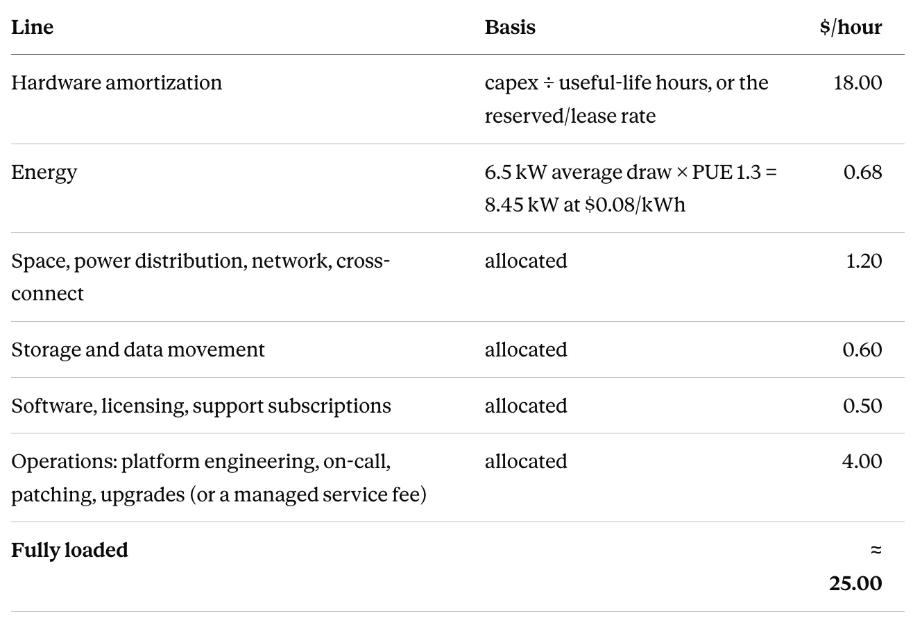
Operations is the easiest line to leave out of a comparison and not necessarily the smallest, since staffing an on-call rotation for a serving platform costs what it costs whether or not it appears on an infrastructure invoice.
Step 2. Achieved throughput at the required service level.
This is the number that decides the whole comparison, and it may not be the one on the benchmark sheet. Peak-throughput figures can be measured under batching or latency conditions that look nothing like your production service level, so check what was held constant before reusing a published number. What you want is what the node sustains while meeting your latency targets on your traffic.
Say you're targeting p95 time to first token at or under 800 ms and p95 inter-token latency at or under 50 ms. Under those constraints, this node completes 3,600 successful outcomes an hour on your workload.
Cost per successful outcome at full achieved throughput = $25.00 ÷ 3,600 = $0.0069
That's roughly half the API figure, though only at full achieved throughput, which is a demanding condition to hold.
Step 3. Break-even, and what demand shape does to it.
Before putting the two side by side, be explicit about what makes them comparable. Both configurations have to clear the same quality bar on the same evaluation set, since a cheaper number produced by a weaker model is a different product rather than a saving. They also have to agree on what counts as a successful outcome, down to retry policy, acceptance criteria and how failures get classified, because if one side counts a partially useful response as a success and the other doesn't, the two denominators aren't the same denominator. And the latency requirement has to hold on both sides, with dedicated throughput measured at the target p95 and the API path meeting that same target in practice, including how it queues under your concurrency.
There's also an asymmetry that's easy to miss. The API side gives you a price and a service level rather than an implementation, so you don't know the provider's hardware, batching strategy or serving configuration, and you aren't buying them. The comparison is still legitimate, but what it compares is delivered outcomes at a given quality and latency rather than like-for-like infrastructure.
With all that held constant:
Break-even volume = $25.00 ÷ $0.0123 = ~2,025 outcomes per hour
That's about 56% of what the node can do. Within the single-node capacity range, dedicated is cheaper from roughly 2,025 to 3,600 outcomes an hour, and below 2,025 the API is cheaper. The comparison has to be redone at every capacity step, because adding a node resets it, as the next section shows.
Now bring in real demand. Twenty thousand outcomes a day averages 833 an hour. If your peak runs 2.5× the mean, that's about 2,083 an hour, which one node covers comfortably.
At the average rate, though: $25.00 ÷ 833 = $0.030 per successful outcome
Around 2.4× the API cost for the same workload at the same quality and latency targets. Nothing here was specified incorrectly; the node is correctly sized for peak, and that's precisely why it looks expensive at the average.
Dedicated inference is often described as a fixed cost plus a marginal cost that approaches zero. That description is wrong in a way that changes decisions.
Inside a node that's already running and not yet saturated, the genuine per-request marginal costs are incremental energy draw plus network and storage I/O, which are small without being zero. Operations doesn't belong in that category at all, since it behaves as a fixed or stepwise cost that moves when you add a node, extend a rotation or take on another failure domain rather than when one more request arrives.
The more consequential point is that marginal cost here isn't smooth. Once a node saturates at your target latency, additional request volume can't be sustained within the target service level. You then have four choices, each carrying a cost that belongs in the model:
Follow that fourth option through. Demand grows to 3,800 outcomes an hour, 200 past what one node delivers, so you add a second:
$50.00 ÷ 3,800 = $0.0132 per successful outcome
That's more than the API's $0.0123, so the economics invert at the step and then recover as the second node fills. Availability headroom pulls the step forward: run N+1 so a node can fail or be patched without breaching your service level, and you'll need the second box well before the first one saturates.
So the crossover between consumption pricing and dedicated capacity doesn't hinge "almost entirely" on sustained utilization. It depends on:
Utilization summarizes several of these at once, which makes it a reasonable headline and a poor substitute for the model underneath.
These are the places cost tends to accumulate, offered as areas to test against your own workload rather than a ranked list, since the order shifts substantially by workflow and a lever that transforms one deployment can do nothing for the next.
Not calling the model. Some portion of production traffic can be handled by a cache, a lookup, a deterministic rule or a small classifier gating access to the large model. How large that portion is depends entirely on the workload, so it's better to measure it than to assume it's either huge or negligible. Where it does exist, it compounds with everything downstream.
Model right-sizing. Selection often happens early, based on a general impression of capability, and never gets revisited as the task narrows. Setting a quality threshold for the specific task and finding the smallest configuration that clears it is a measurable exercise, though only with an evaluation set that reflects real traffic. Tiered routing, where most requests hit a smaller model and only hard cases escalate, is the practical version of the same idea.
Quantization. Reduced-precision weights can shrink the memory footprint and raise throughput, which changes how many requests fit on a device. The effect on quality and latency is specific to your model, hardware and task, so treat published quality deltas as a prompt to run your own evaluation rather than a substitute for one.
Prompt and context discipline. Input tokens cost money, and input counts grow without anyone deciding they should. Retrieval tuned for recall returns more chunks than actually influence the answer, system prompts accumulate instructions nobody has audited in months, and full conversation history gets resent when a summary would carry the same information. Output length deserves the same attention, since output tokens are often priced above input tokens and are generated sequentially, which usually gives them a heavier cost and latency weight per token, though the ratio varies by provider, model and deployment and is worth checking against your own.
Prefix caching. Caching a shared prompt prefix avoids recomputing it, but only where prefixes repeat at the granularity the cache operates on. vLLM's automatic prefix caching hashes fixed-size blocks of the KV cache and reuses them across requests that share a prefix, so the benefit approaches zero when no full blocks repeat (vLLM prefix caching design). That's a stricter condition than prompts simply not being identical, because two prompts can share a long opening and still return nothing if the shared span falls short of a block, or if variable content appears early enough to break block alignment. Putting the stable portion first and making it long enough to fill blocks is what makes the mechanism available at all; the hit rate is what tells you whether it's doing anything.
Batching and concurrency. Continuous batching admits new requests as others finish instead of waiting for a fixed batch to fill, which generally improves device productivity and can reduce queueing compared with static batching, though it doesn't eliminate the underlying tradeoff. Batch size, maximum concurrent sequences and KV cache capacity together place a deployment somewhere on a throughput-versus-latency curve, and that curve belongs to your workload, so tune against your own p95 TTFT and inter-token latency rather than a default or someone else's published number (vLLM optimization guidance). KV cache capacity also determines how many requests run concurrently before the scheduler starts preempting work already in flight.
There's a widely repeated line that prefill is compute-bound and decode is memory-bandwidth-bound. As a first approximation that's often true and it usefully explains why the two phases behave differently, but it describes a tendency rather than a rule. Which resource binds depends on model architecture, the hardware's compute-to-bandwidth ratio, batch size and context length. Decode can become compute-bound at large batch sizes, and very long contexts change the picture again once attention over the KV cache starts to dominate.
The practical consequence survives all of that. Long inputs with short outputs, as in classification, extraction and summarization, have a different cost and latency profile from short inputs with long outputs, as in content generation, so a serving configuration tuned for one can be a poor fit for the other. That's the argument for measuring your own input-to-output ratio rather than importing someone else's conclusion.
None of the decisions above can be made defensibly without instrumentation, and the metrics below are roughly the floor. NVIDIA's LLM benchmarking fundamentals and its NIM benchmarking metric definitions are useful for pinning down definitions first, since inconsistent ones can make two throughput figures impossible to compare.
Metrics and what they tell you
Time to first token (TTFT)
Queueing plus prompt processing, and depending on where you draw the measurement boundary, tokenization, network transit and frontend overhead. Fix the boundary before comparing any two figures
Inter-token latency / time per output token
Decode performance; what the user perceives as generation speed
End-to-end request latency
The number your service level is actually written against
Output token throughput (tokens/sec)
Capacity for generation-heavy workloads
Input token throughput (tokens/sec)
Capacity for prefill-heavy workloads such as RAG, long-context, classification and extraction, where output throughput understates the work being done
Request throughput (requests/sec)
A key denominator for request- and outcome-based cost calculations; record it at the target latency, not under peak-throughput conditions
Queue time
Whether you're capacity-constrained rather than slow
Effective batch size
Whether batching is doing anything under real traffic
KV cache utilization and preemption rate
Whether concurrency limits are forcing the system to throw away partial work
Prefix cache hit rate
Whether caching is delivering on your actual prompt distribution
Cost per attempt, split by input and output tokens
Which side of the workload to go after
Cost per successful outcome
Primary unit-economics figure; read alongside total spend and service-level performance
vLLM exposes most of the serving-side metrics natively through Prometheus, including TTFT, time per output token, end-to-end latency, queue time and cache usage (vLLM metrics design). Report latency as distributions rather than averages, since a mean TTFT says almost nothing about what happens at p95, and p95 is where service levels break.
Quite often, and any honest treatment of the topic has to say so.
If your volume is modest or unpredictable, if the provider's data handling and regional terms already satisfy your requirements, if latency isn't tightly constrained and if you have no obligations about where processing happens or which model runs, then a consumption-priced API may well be the right answer, and standing up a serving platform to avoid it would be hard to justify on cost alone.
The answer changes when the numbers cross, or when a constraint appears that was never financial in the first place: a security or contractual review restricting where data can be processed, a model or configuration the provider doesn't offer, latency requirements that demand control of the serving path, or a need to switch models without renegotiating the architecture. Constraints like these often settle the placement question before economics gets a vote, which is why they belong in the model from the start rather than arriving late as an objection.
The last question tends to reframe the rest of them. An optimization that welds your architecture to a single provider or model can be painful to unwind, and the conditions that made it cheap rarely stay put.
We treat model selection, serving configuration and placement as one decision rather than three separate purchases. Managed AI Inference gives you an endpoint we deploy, monitor and operate, running open, commercial or custom model paths, hosted in a VEXXHOST data centre or on GPU infrastructure in yours, so that placement follows from what the workload needs rather than from what happens to be easiest to buy.
If the model above points you toward dedicated capacity, GPU Infrastructure covers the layer beneath it: workload-sized compute, storage, network and control plane, in our facilities or on your own hardware, with support or managed operations depending on which layers your team wants to keep. Residency, retention and model-control constraints shape that design up front rather than surfacing as a problem after launch.
The useful starting point is the two models above, filled in with your own numbers.
Related reading
Choose from Atmosphere Cloud, Hosted, or On-Premise.
Simplify your cloud operations with our intuitive dashboard.
Run it yourself, tap our expert support, or opt for full remote operations.
Leverage Terraform, Ansible or APIs directly powered by OpenStack & Kubernetes